10
The theory of normal forms is concerned with the structure of relations in a relational database. There are several normal forms of which 1NF, 2NF, 3NF and Boyce-Codd (BCNF) are the most important for practical online transaction processing (OLTP) database design. Online transaction processing (OLTP) systems are used to run the day-to-day events of a business.
Normalization theory gives us a theoretical basis to judge the quality of a database and helps one understand the impact of some design decisions. In practice, Entity Relationship Modeling is the primary technique used for designing databases and experienced practitioners will typically develop BCNF relations as a result. Normalization can be applied by the practitioner to understand better the semantics behind some relations and possibly make some design modifications.
Boyce-Codd (1NF – 3NF)
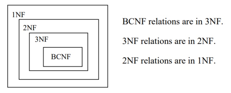
1NF, 2NF, 3NF and BCNF are acronyms for first normal form, second normal form, third normal form, and Boyce-Codd normal forms. There is a sequence to normal forms: 1NF is considered the weakest, 2NF is stronger than 1NF, 3NF is stronger than 2NF, and BCNF is considered the strongest of these four normal forms. Also, any relation that is in BCNF, is in 3NF; any relation in 3NF is in 2NF; and any relation in 2NF is in 1NF. This correspondence can be shown as:
Transactions are units of work designed to meet the goals of users. For instance in a banking environment, we would expect to find a deposit transaction, a withdrawal transaction, a transfer transaction, and a balance lookup transaction. A unit of work is a collection of database operations that are executed in their entirety or not at all. For example, if you are transferring money from one account to another, it’s important for the integrity of accounts that the transfer be completely done, and never partly done. If a transfer transaction is partly done (say, because of a system failure) then accounts would be out of balance. A database environment has capabilities to back out partly executed transactions so the system can be back where it was prior to a failed transfer transaction. A banking system could have thousands of users and we expect transactions such as these to be correctly and efficiently executed. A normalized database is such that every relation is in at least 1NF, and preferably 3NF. Generally speaking, normalized databases lead to the most efficient designs for these types of transactions.
Normalization
Normalization is a process that replaces a relation with other relations of a higher normal form. The process involves decomposing a relation into other relations in such a way as to preserve the original information and reduce redundancy of data. Reducing redundant data increases the number of relations, but makes the data easier to maintain. Later, we will provide examples of decomposition.
We say normalization is a process that improves a database design. The objective of normalization is sometimes stated: to create relations where every dependency is on the key, the whole key, and nothing but the key[1]. A relation that is fully normalized is about a single concept such as a student entity type, a course entity type, and so on.
De-normalization is a process that changes relations from higher to lower normal forms, and hence generates redundant data in the tuples (rows/records) of a relation (table). If deemed necessary, this would be done to improve the performance (reduce the cost) of retrieving information from the database. The cost of querying de-normalized relations is generally less because fewer joins are required.
We consider higher normal forms to be better choices because the update semantics for data are simplified. By this, we mean that applications required to maintain the database are simpler to code and so they are easier to maintain. In the following, we discuss:
- Functional Dependencies
- Update Anomalies
- Partial Dependencies
- Transitive Dependencies
- Normal Forms
10.1 Functional Dependencies
To understand normalization theory (first, second, third and Boyce-Codd normal forms), we must understand what is meant by the term functional dependency. There is another type of dependency called a multi-valued dependency, but that is important to the understanding of higher normal forms not covered in this text. A functional dependency is an association between two attributes. We say there is a functional dependency from attribute A to an attribute B if and only if for each value of A there can be at most one value for B. We can illustrate this by writing
- A functionally determines B, or
- B is functionally determined by A, or
- by a drawing such as:
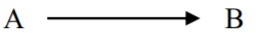
When we have a functional dependency from A to B we refer to attribute A as the determinant.
Example 1
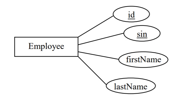
Consider a company collecting information about each employee such as the employee’s identification number (ID), their first name, last name, salary and gender. As is typical, each employee is given a unique ID which serves to identify the employee. Hence for each value of ID, there is at most one value for first name, last name, salary and gender. Therefore, we have four functional dependencies where ID is the determinant; we can show this as a list or graphically:
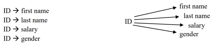
If you think about this case, there cannot be any other functional dependencies (FDs). For example, consider the gender attribute – we need to allow for more than one employee for a given gender, and so we cannot have a situation where gender functionally determines ID. So, gender ![]() ID cannot exist. Now consider the first name attribute. Again, we need to allow for more than one employee to have the same first name and so first name cannot determine anything. Similarly for other attributes.
ID cannot exist. Now consider the first name attribute. Again, we need to allow for more than one employee to have the same first name and so first name cannot determine anything. Similarly for other attributes.
Example 2
Recall the Department and Course tables introduced in Chapter 2 – sample data is shown below:
| Department | |||||
| deptCode | deptName | deptLocn | deptPhone | chairName | |
| ENGL | English | 3D05 | 786-9999 | April Jones | |
| MATH | Mathematics | 2R33 | 786-0033 | Peter Smith | |
| ACS | Applied Computer Science | 3D07 | 786-0300 | Simon Lee | |
| PHIL | Philosophy | 3C11 | 786-3322 | Judy Chan | |
| BIOL | Biology | 2L88 | 786-9843 | James Dunn | |
Figure 2.1 Department table
| Course | |||||
| deptCode | courseNo | title | description | creditHours | |
| ACS | 1453 | Introduction to Computers | This course will introduce students to the basic concepts of computers: types of computers, hardware, software, and types of application systems. | 3 | |
| ACS | 1803 | Introduction to Information Systems | This course examines applications of information technology to businesses and other organizations. | 3 | |
| ENGL | 2221 | The Age of Chaucer | This course examines a selection of medieval poetry and drama with emphasis upon Chaucer’s Canterbury Tales. |
6 | |
| PHIL | 2219 | Philosophy of Art | Through reading key theorists in the history of esthetics, this course examines some of the fundamental problems in the philosophy of art, including those of the definition and purpose of art, the nature of beauty, the sources of genius and originality, the problem of forgery, and the possible connection between art and the moral good | 3 | |
| BIOL | 4451 | Forest Ecosystems Field Course | This is an intensive three-week field course designed to give students a comprehensive overview of forest ecology field skills. | 2 | |
| BIOL | 4931 | Immunology | Immunology is the study of the defense system which the body has evolved to protect itself from external threats such as viruses and internal threats such as tumor cells. | 3 | |
Figure 2.2 Course table
Recall the primary keys (underlined above) of these two tables:
|
Table |
Primary Key |
|
Department |
deptCode |
|
Course |
deptCode, courseNo |
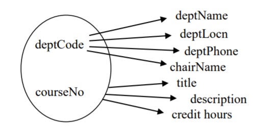
Consider the Department table where deptCode is the primary key. For each value of deptCode, there is at most one value for deptName, deptLocn, deptPhone, and chairName. You should agree the following functional dependencies exist:
deptCode ![]() deptName
deptName
deptCode ![]() deptLocn
deptLocn
deptCode ![]() deptPhone
deptPhone
deptCode ![]() chairName
chairName
Each row of the Course table has one value for title, one value for description, and one value for credit hours. The primary key of Course is consists of two attributes, deptCode and courseNo.
The following functional dependencies exist for the Course table:
deptCode, courseNo ![]() title
title
deptCode, courseNo ![]() description
description
deptCode, courseNo ![]() credit hours
credit hours
In this case, we have a determinant comprising two attributes; the determinant is composite.
We can draw the functional dependencies as:
Could there be other functional dependencies in this situation?
These examples demonstrate that there is a functional dependency from the primary key to each of the other attributes in a table.
Example 3.
The following entity relational diagram (ERD) is shown in the Chen notation. There is one entity type named Employee that has 4 attributes. In this design, there are two keys (id and sin) and two descriptive attributes (firstName and lastName)
Each symbol in an ER diagram contains information about a model. From the above, we know there are two keys – id and sin. An id value, or a sin value, will uniquely identify an employee and so we have the six functional dependencies (FDs):
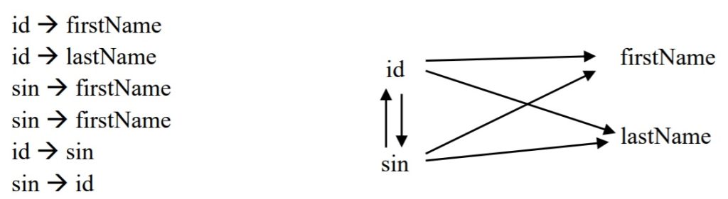
This example shows that an ER Diagram carries information that can be expressed in terms of functional dependencies.
Exercises
- Consider the Product table below where productID is the PK. What FDs must exist in this table:
productID
description
unit price
quantity on hand
33
16 oz. can tomato soup
1.00
50
41
454 gram box corn flakes
4.50
39
45
Package red licorice
1.00
39
46
Package black licorice
1.00
50
47
1 litre 1% milk
1.99
25
- Consider the ERD where the entity type Employee has one key attribute, id, and the entity type Position has one key attribute, title. As well the ERD shows a one-to- many relationship assigned to which can be expressed as:
An employee is assigned to at most one position.
A position can be assigned to many employees.
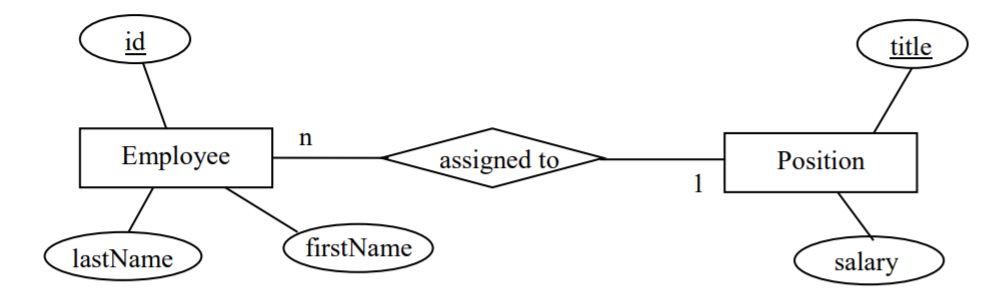
List the FDs that must be present.
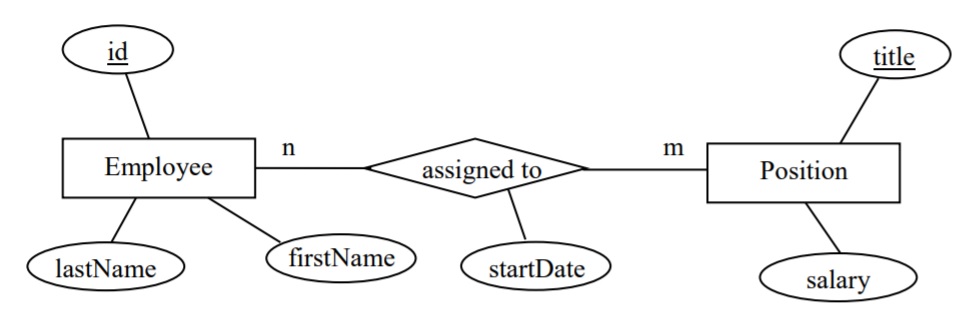
- Consider this ERD that is similar to the above but where the assigned to relationship is many-to-many, and where assigned to has an attribute startDate. List the FDs that are present.
- Consider the ERD below where Department has two keys deptCode and deptName – each department has a unique department code and has a unique department name. Course is a weak entity type with a partial key courseNo, and where offers is an identifying relationship.
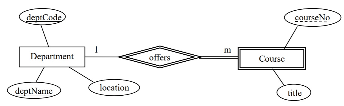
List the FDs that must exist.
- Consider the table with attributes A, B and C.
|
A |
B |
C |
|
1 |
33 |
100 |
|
2 |
33 |
200 |
|
3 |
22 |
200 |
|
1 |
33 |
101 |
|
2 |
33 |
350 |
|
4 |
67 |
350 |
|
5 |
67 |
101 |
Suppose there are many more rows that are not shown.
a) Is there a functional dependency from B to A? Explain your answer.
b) The rows that are shown suggest there could be a functional dependency A ![]() B. Compose a database query that would list rows, if they exist, that are counterexamples to the functional dependency A
B. Compose a database query that would list rows, if they exist, that are counterexamples to the functional dependency A ![]() B. Such a query would list rows in the table where two or more rows have the same value for A but different values for B.
B. Such a query would list rows in the table where two or more rows have the same value for A but different values for B.
10.1.2 Keys and Non-Keys
Before going further, we need to be clear regarding the concept of key. We define the key of a relation to be any minimal set of attributes that uniquely identify tuples in the relation. We say minimal in order to eliminate trivial cases. Consider: If attribute k is a key and uniquely identifies a tuple then any combination of attributes that include k must also uniquely identify tuples. So, we restrict keys to be minimal sets of attributes that retain the property of unique identification. Further, we define candidate keys to be the collection of keys for a relation; a database designer must choose one of the candidate keys to be the primary key.
Additionally, we define key attributes to be those attributes that are part of a key, and non-key attributes are those attributes that are not part of any key.
10.1.3 Anomalies
An anomaly is a variation that differs in some way from what is considered normal. With regards to maintaining a database, we consider the actions that must occur when data is updated, inserted, or deleted. In database applications where these update, insert, and/or delete operations are common (e.g. OLTP databases), it is desirable for these operations to be as simple and efficient as possible.
When relations are not fully normalized, they exhibit update anomalies because basic operations are not as simple as possible. When relations are not fully normalized, some aspect of the relation will be awkward to maintain.
Consider the relation structure and sample data:
|
deptNum |
courseNum |
studNum |
grade |
studName |
|
92 |
101 |
3344 |
A |
Joe |
|
92 |
115 |
7654 |
A |
Brenda |
|
81 |
101 |
7654 |
C |
Brenda |
|
92 |
226 |
3344 |
B |
Joe |
This relation is used for keeping track of students enrollments, the grade assigned, and (oddly) the student’s name.
What must happen if a student’s name were to change? We should want our databases to have correct information, and so the name may need to be changed in several records, not just one. This is an example of an update anomaly – the simple change of a student’s name affects, not just one record, but potentially several in the database. The update operation is more complex than necessary, and this means it is more expensive to do, resulting in slower performance. When operations become more complex than necessary, there is also a chance the operation is programmed incorrectly resulting in corrupted data – another unfortunate consequence.
Consider the Course and Department tables again, but now consider that they are combined into a single table. Obviously, this is a table with a considerable redundancy – for each course in the same department, the department location, phone, and chair must be repeated.
|
Department_Course |
||||||||
|
dept Code |
dept Name |
dept Location |
dept Phone |
chair Name |
course No |
title |
description |
credit Hours |
The primary key of such a table must be {deptCode, courseNo}. Consider for the following, however unlikely the situation seems, that the Deparment_Course table is the only table where department information is kept. Note that our point here is only to show, for a simple example, how redundancy leads to difficult semantics for database operations.
Insert anomaly
Suppose the University added a new department but there are no courses for that department yet. How can a row be added to the above table? Recall that no part of a primary key can be null, and so we can’t insert a row for a new department because we do not have a value for courseNo. This is an example of an insertion anomaly.
Delete anomaly
Suppose some department is undergoing a major reorganization. All courses are to be removed and later on some new courses will be added. If we delete all courses then we lose all the information in the database for that department.
The previous discussion concerning anomalies highlights some of the data management issues that arise when a relation is not fully normalized. Another way of describing the general problem here, as far as updating a database is concerned, is that redundant data makes it more complicated for us to keep the data consistent.
10.1.4 Partial Functional Dependencies
Consider a relation with department number, department chair name, course number and course title attributes. The combination {department number, course number} must be a key. The directed lines depict the FDs that are present.
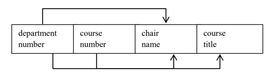
Note the functional dependency of chair name on department number. If two or more rows in the relation have the same value for department number, they must have the same value for chair name. We say this redundancy is due to the FD of chair name on department number. Because chair name is a non-key attribute and is dependent on department number, a subset of a key, we call this dependency a partial dependency.
In general, if we have a composite key {A, B} and the dependencies below
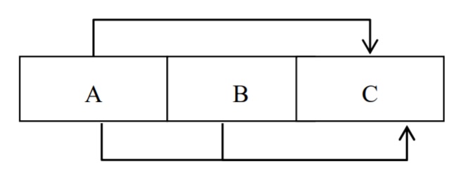
we say that C is partially dependent on {A, B}.
Exercises
- Suppose each delivery of a course is called a section. In any one term, a course may have multiple sections and each section is assigned an instructor. Each course has a course title. Consider a Section relation where the PK is {dept number, course number, section number}. What FDs exist? Is there a partial dependency?
deptNo
courseNo
sectionNo
instructor
title
91
1906
001
J. Smith
Java I
91
1906
002
D. Grand
Java I
91
1910
001
J. Smith
Java II
91
1910
002
J. Daniels
Java II
53
1906
001
S. Farrell
History of the World
…
…
…
…
…
- Consider a relation with attributes X, Y, Z, W where the only CK is {X,Y}, and where the FDs are {X,Y}
 Z, {X,Y} W, and Y W. Is there a partial dependency?
- Consider a relation with attributes X, Y, Z, W where the only CK is {X,Y}, and where the FDs are {X,Y}
10.1.6 Transitive Functional Dependencies
Consider a relation that describes a couple of concepts, say instructor and department, and where the building shown is the building where the department is located, and the attribute instructor number is the only key:
|
instructor number |
instructor name |
office |
department code |
building |
|
33 |
Joe |
3D15 |
B&A |
Buhler |
|
44 |
Joe |
3D16 |
ACS |
Duckworth |
|
45 |
April |
3D17 |
ACS |
Duckworth |
|
50 |
Susan |
3D17 |
ACS |
Duckworth |
|
21 |
Peter |
3D18 |
B&A |
Buhler |
|
22 |
Peter |
3D18 |
MATH |
Duckworth |
As instructor number is the only key, we have the following FDs:
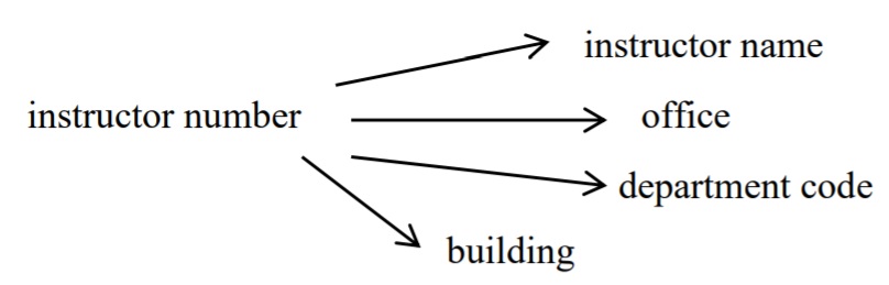
Suppose we also have the FD: department code determines building. Now our FD diagram becomes:
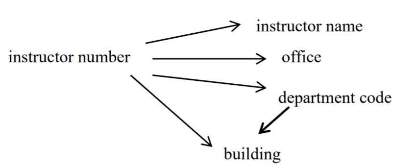
and we say the FD from instructor number to building is transitive via department code.
In general, if we have a relation with key A and functional dependencies: A ![]() B and B
B and B ![]() C, then we say attribute A transitively determines attribute C.
C, then we say attribute A transitively determines attribute C.
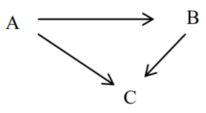
Figure 10.9 Non-key attributes and a transitive dependency
Note: B and C above are non-key attributes. If we also had the functional dependency B ![]() A (and so A and B are candidate keys) then A does not transitively determine C.
A (and so A and B are candidate keys) then A does not transitively determine C.
Exercises
- Consider a relation that describes an employee including the province where the employee was born. Suppose the only key is employeeId and we have the attributes: name, birthDate, birthProvince, currentPopulation.
Employee
employeeId
name
birthDate
birthProvince
currentPopulation
123
Joe
Jan 1, 1990
MB
1,200,000
222
Jennifer
Jan 5, 1988
SK
1,450,000
345
Jimmy
Feb 5, 1987
MB
1,200,000
…
…
…
…
…
What FDs would exist? Is there a transitive dependency?
- Consider a relation with attributes X, Y, Z, W where the only CK is X, and the FDs are X Y, X Z, X W and Y Z. Is there a transitive dependency?
Normal Forms
The normal forms usually of interest to the database designer are 1NF, 2NF, 3NF and BCNF. There are more (higher) normal forms that we leave to follow-up courses. We discuss 1NF and BCNF; 2NF and 3NF are mentioned in our summary. 1NF is so important, it is actually a property of a relation; that is, to say something is a relation means that it is at least in 1NF. BCNF has a simple definition (compared to 2NF and 3NF) and is the usual objective of the designer.
If you understand 1NF and BCNF then you have good insight into the nature of relations that are easy to understand and maintain. If you understand why a relation is not BCNF then you will know the source of its redundant data which is necessary in order to know how to properly maintain the data contained in the relation. In most practical cases when a relation is not BCNF, the reason will be related to partial or transitive dependencies. 2NF relations do not have partial dependencies, and 3NF relations do not have partial nor transitive dependencies.
10.2 FIRST NORMAL FORM (1NF)
We say a relation is in 1NF if all values stored in the relation are single-valuedand atomic. With this rule, we are simplifying the structure of a relation and the kinds of values that are stored in the relation.
Example 1
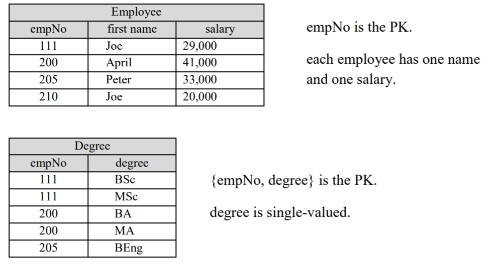
Consider the following EmployeeDegrees relation.
-
- empNo is the PK
- Each employee has one first name and one salary
- Each employee has zero or more university degrees … stored as a single attribute
|
EmployeeDegrees |
|||
|
empNo |
first name |
salary |
degrees |
|
111 |
Joe |
29,000 |
BSc, MSc |
|
200 |
April |
41,000 |
BA, MA |
|
205 |
Peter |
33,000 |
BEng |
|
210 |
Joe |
20,000 |
|
This relation is not in 1NF because the degrees attribute can have multiple values. Below are two relations formed by splitting EmployeeDegrees into two relations – one relation has attributes empNo, first name, and salary and the other has empNo and degree. We say we have decomposed EmployeeDegrees into two relations and we have populated each with data from EmployeeDegrees. Each of these is in 1NF, and if we join them on empNo we can get back the information shown in the relation above.
Example 2
Consider the Student relation below. The name attribute comprises both first and last names and so its not atomic. Student is not 1NF.
|
Student – not in 1NF |
||
|
studentNo |
name |
gender |
|
444 |
Jim Smith |
m |
|
254 |
Donna Jones |
f |
|
333 |
Peter Thomas |
m |
|
765 |
Jim Smith |
m |
If we modify Student so there are two attributes (say, first and last) then Student would be 1NF:
|
Student – in 1NF |
|||
|
studentNo |
first |
last |
gender |
|
444 |
Jim |
Smith |
m |
|
254 |
Donna |
Jones |
f |
|
333 |
Peter |
Thomas |
m |
|
765 |
Jim |
Smith |
m |
If we can say that a relation (or table) is in 1NF then we are saying that every attribute is atomic and every value is single-valued. This simplifies the form of a relation.
It is very common for names to be separated out into two or more attributes. However, attributes such as birth dates, hire dates, etc. are usually left as a single attribute. Dates could be separated out into day, month, and year attributes, but that is usually beyond the needs of the intended system. Some would take the view that separating a date into 3 separate attributes is carrying the concept of normalization a little too far. Database systems do have convenient functions that can be used to obtain a day, month, or year values from a date.
10.2 Exercises
- Consider the relation below that holds information about courses and sections. Suppose departments have courses and offer these courses during the terms of an academic year. A section has a section number, is offered in a specific term (e.g. Fall 2016, Winter 2017) and a slot (e.g. 1, 2, 3, …15) within that term. Each time a course is delivered, there is a section for that purpose. Each section of a course has a different number. As you can see, a course may be delivered many times in one term.
CourseDelivery
deptNo
courseNo
delivery
ACS
1903
001, Fall 2016, 05;
002, Fall 2016, 06;
003, Winter 2017, 06
ACS
1904
001, Fall 2016, 12;
002, Winter 2017, 12
Math
2201
001, Fall 2016, 11;
050, Fall 2016, 15
Math
2202
050, Fall 2016, 15
Modify CourseDelivery to be in 1NF. Show the contents of the rows for the above data.
- Chapter 8 covered mapping an ERD to a relational database. Consider the examples from Chapter 8; are the relations in 1NF?
10.3 Boyce-Codd Normal Form (BCNF)
Initial research into normal forms led to 1NF, 2NF, and 3NF, but later[2] it was realized that these were not strong enough. This realization led to BCNF which is defined very simply:
A relation R is in BCNF if R is in 1NF and every determinant of a non-trivial functional dependency in R is a candidate key.
BCNF is the usual objective of the database designer, and is based on the notions of candidate key (CK) and functional dependency (FD). When we investigate a relation to determine whether or not it is in BCNF, we must know what attributes or attribute combinations are CKs for the relation, and we must know the FDs that exist in the relation. Our knowledge of the semantics of a relation guides us in determining CKs and FDs.
Recall that a CK is an attribute, or attribute combination, that uniquely identifies a row. Also, recall a CK is minimal – no attribute can be removed without losing the property of being a key.
Recall that a FD X ![]() Y in a relation R means that for each row in the relation R that has the same value for X the value of Y must also be the same.
Y in a relation R means that for each row in the relation R that has the same value for X the value of Y must also be the same.
Recall that when we consider a FD X ![]() Y we refer to the left hand side, attribute X, as the determinant. We are concerned with minimal FDs – all attributes comprising the determinant are required for the FD property to hold. If X
Y we refer to the left hand side, attribute X, as the determinant. We are concerned with minimal FDs – all attributes comprising the determinant are required for the FD property to hold. If X ![]() Y is a FD then the determinant augmented with any other attribute is also a FD, but it would not be a minimal FD.
Y is a FD then the determinant augmented with any other attribute is also a FD, but it would not be a minimal FD.
We consider a number of examples. The keep the examples simple and to the point, each relation involves very few attributes. This is of course unrealistic – in practice relations usually have many attributes. However, the examples illustrate one point each, and more attributes in the relations may cloud the issues. Each example begins with a relation that is in 1NF.
In general, when we determine the relation under consideration is not in BCNF, we obtain BCNF relations by decomposing the relation into two or more relations that are in BCNF. In this process, we say we take a projection of the original relation on a subset of its attributes and at the same time we eliminate any duplicate rows. An important property of the decomposition is that it must be lossless – the new relations will have attributes in common that can be used to join the new relations whereby we can realize the original relation. All rows of the original relation are obtained in the join, and no new or spurious rows are generated – we get back the original relation exactly.
In Example 1, we have a ‘good’ relation, one that is in BCNF. Hence, no decomposition is required. We discuss the CDs and FDs for the relation thereby knowing it is in BCNF.
Example 2 presents a relation that is not in BCNF. There is a type of redundancy present in its data. We illustrate how to decompose the relation into two relations that are each in BCNF. This example illustrates a type of dependency known as a partial functional dependency.
Example 3 presents another relation that is not in BCNF. There is a type of redundancy present in its data. We illustrate how to decompose the relation into two relations that are each in BCNF. This example illustrates a type of dependency known as a transitive functional dependency.
Our last example is a case where FDs involve overlapping candidate keys, and where FDs exist amongst attributes that make up CKs. There is a type of redundancy present which is not related to 2NF and 3NF. BCNF gives us a theoretical basis for recognizing the source of the redundant data.
Example 1
Consider the Employee relation below that depicts sample data for 5 employees. The semantics are quite simple: for each employee identified by a unique employee number, we store the employee’s first name and last name.
|
Employee |
||
|
id |
first |
last |
|
1 |
Joe |
Jones |
|
2 |
Joe |
Smith |
|
3 |
Susan |
Smith |
|
4 |
Abigail |
McDonald |
|
5 |
Abigail |
McDonald |
Candidate Keys
The hypothetical company that uses this relation identifies employees by an identification number that is assigned by the Human Resources Department and they ensure each employee has a different id from every other employee. Clearly id is a candidate key. When an employee is hired they have a first and last name, and the company has no control over these names. As the sample data shows, more than one employee can have the same first name (id 1 and 2), can have the same last name (id 2 and 3), and can even have the same first and last names (id 4 and 5).
So, id is the only candidate key for this relation.
Functional Dependencies
Since each row/employee has a unique identifier, it is easy to see there are two FDs for this relation:
id ![]() first
first
id ![]() last
last
There are no other FDs. For example, we cannot have first ![]() last. The sample data shows there can be many last names associated with any one first name.
last. The sample data shows there can be many last names associated with any one first name.
These two FDs are minimal as the determinant, id, cannot be reduced at all.
BCNF?
In this example, we have one candidate key, id, and this attribute is the determinant in all FDs. Therefore, Employee relation is in BCNF; it is a ‘good’ relation.
This relation has a ‘nice’ simple structure; there is one candidate key which is the determinant for every FD.
Example 2
Consider the following relation named Enrollment:
|
Enrollment |
||
|
stuNum |
courseId |
birthdate |
|
111 |
2914 |
Jan 1, 1995 |
|
113 |
2914 |
Jan 1, 1998 |
|
113 |
3902 |
Jan 1, 1998 |
|
118 |
2222 |
Jan 1, 1990 |
|
118 |
3902 |
Jan 1, 1990 |
|
202 |
1805 |
Jan 1, 2000 |
The semantics of this relation are:
- Each row represents an enrollment of a student in a course.
- A student is identified by their student number.
- A course is identified by a course identifier.
- A student can only enroll in a course once. Hence the combinations {stuNum,courseId} are unique.
- The birthdate column holds the date of birth for the student of that row. When the same student number appears in more than one row then the birthdate appears redundantly.
- A course can have many students registered in it
Candidate Keys
It should be clear that several rows may exist for any given student number, and several rows may exist for any given course number. Also, since we cannot control when someone is born, there can be many rows for a value of birthdate. All this just means that no single attribute uniquely identifies a row and so no single attribute can be a CK. Any CKs for this relation must be composite – comprising more than one attribute. It should be fairly clear, given the semantics of the relation, that the only attribute combination that is a CK is {stuNum,courseId}. For any given value of {stuNum, courseId} there can be at most one row.
Functional Dependencies
This relation is quite simple in that there is just one FD: stuNum ![]() birthdate. If a specific student number appears in more than one row, the value stored for birthdate must be the same in all such rows.
birthdate. If a specific student number appears in more than one row, the value stored for birthdate must be the same in all such rows.
BCNF?
Enrollment has one CK: {stuNum, courseId}, and has one FD (stuNum ![]() birthdate) where the determinant is not a candidate key. Therefore, Enrollment is not in BCNF.
birthdate) where the determinant is not a candidate key. Therefore, Enrollment is not in BCNF.
In this relation, we have an attribute that does not describe the whole key – it describes a part of the key. In normalization theory, the FD stuNum ![]() birthdate is called a partial functional dependency as its determinant is a subset of a candidate key.
birthdate is called a partial functional dependency as its determinant is a subset of a candidate key.
When you think of the Enrollment relation now, you should consider that it is about two very different things:
- Enrollment presents enrollment information.
- Enrollment presents information about students (their birthdates).
Decomposition
We now consider how Enrollment can be replaced by two relations where the new relations are each in BCNF. Above, we mentioned that Enrollment is about two very different things – what we need to do is arrange for two relations, one for each of these concerns.
Consider the following two relations as a decomposition of the above where we have placed information about enrollments in one relation and information about students in another relation. Note that these two relations have the stuNum attribute in common.
|
Enrollments |
|
|
stuNum |
courseId |
|
111 |
2914 |
|
113 |
2914 |
|
113 |
3902 |
|
118 |
2222 |
|
118 |
3902 |
|
202 |
1805 |
|
Students |
|
|
stuNum |
birthdate |
|
111 |
Jan 1, 1995 |
|
113 |
Jan 1, 1998 |
|
118 |
Jan 1, 1990 |
|
202 |
Jan 1, 2000 |
Enrollments and Students can be joined on stuNum to reproduce the exact information in Enrollment. Because we have not lost any information, and noting that the FD has been preserved, these two relations are equivalent to the one we started with.
- Enrollments has one candidate key: {stuNum,courseId}, and no FDs.
Therefore, Enrollments is in BCNF.
Students has one CK: stuNum, and has one FD: stuNum ![]() birthdate.
birthdate.
Therefore, Students is in BCNF.
Example 3
Consider the following relation named Course.
|
Course |
||
|
courseId |
teacherId |
lastName |
|
2914 |
11 |
Smith |
|
3902 |
22 |
Jones |
|
3913 |
11 |
Smith |
|
4902 |
33 |
Jones |
|
4906 |
11 |
Smith |
|
4994 |
22 |
Jones |
The purpose of this relation is to record who is teaching courses. Note that a teacher’s id and last name may appear in several rows – this information is repeated for each course the teacher is teaching. For example, teacher 11 (Smith) is teaching 3 courses (2914, 3913, 4906) and so we see the same id and last name in three rows.
The semantics of this relation are:
-
- Each course is identified by a course identifier.
- For each course there is one row.
- Each teacher is identified by a teacher identifier.
- Each course has one teacher, and so for each course one teacher Id is recorded.
- A teacher may teach several courses.
- A teacher’s last name must be the same in every row where the teacher’s Id appears. This point leads to redundant data in the relation.
Candidate Keys
The semantics of the relation are that there is one row per course, and so a course id uniquely identifies a row; so, courseId is a candidate key. No other attribute or combination can be a candidate key for this relation.
Functional Dependencies
It is stated there is one teacher per course and so for each courseId there is at most one teacherId, and so we have courseId ![]() teacherId. The opposite, teacherId
teacherId. The opposite, teacherId ![]() courseId, does not hold for this relation since a teacher can teach more than one course.
courseId, does not hold for this relation since a teacher can teach more than one course.
Another FD that is present is teacherId ![]() lastName. This is because for each teacher there is a single last name. Note the opposite, lastName
lastName. This is because for each teacher there is a single last name. Note the opposite, lastName ![]() teacherId does not hold in this relation. The sample data shows multiple teachers who have the same last name.
teacherId does not hold in this relation. The sample data shows multiple teachers who have the same last name.
Note that since courseId ![]() teacherId and teacherId
teacherId and teacherId ![]() lastName, it must be true we have the FD courseId
lastName, it must be true we have the FD courseId ![]() lastName. For each course, we have one teacher and so one last name. For any value of course id, there will only be one value for teacher last name. In relational database theory, the FD courseId
lastName. For each course, we have one teacher and so one last name. For any value of course id, there will only be one value for teacher last name. In relational database theory, the FD courseId ![]() lastName is called a transitive functional dependency – lastName is dependent on courseId but this dependency is via teacherId.
lastName is called a transitive functional dependency – lastName is dependent on courseId but this dependency is via teacherId.
BCNF?
Hopefully, you agree the only FDs are these:
- courseId teacherId
- teacherId lastName
- courseId lastName
The only candidate key is courseId, and there is a FD, teacherId ![]() lastName, where the determinant is not a candidate key. Therefore, Course is not BCNF.
lastName, where the determinant is not a candidate key. Therefore, Course is not BCNF.
When you think of the Course relation now, you should see that it is about two very different things:
- Course presents teacher information (teacherId) for courses.
- Course presents information about teachers (their last names).
Decomposition
Course can be replaced by two relations where the new relations are each in BCNF. Above, we mentioned that Course is about two very different things – what we need to do is arrange for two relations, one for each of these concerns.
Consider the following two relations as a decomposition of the above where we have placed information about courses in one table and information about teachers in another table. These relations have a common attribute, teacherId.
|
Courses |
|
|
courseId |
teacherId |
|
2914 |
11 |
|
3902 |
22 |
|
3913 |
11 |
|
4902 |
33 |
|
4906 |
11 |
|
4994 |
22 |
|
Teachers |
|
|
teacherId |
lastName |
|
11 |
Smith |
|
22 |
Jones |
|
33 |
Jones |
Courses and Teachers can be joined on teacherId to reproduce exactly the information in Course. Because we have not lost any information, and noting that the FD has been preserved as well, these two relations are equivalent to the one we started with.
- Courses has one candidate key: courseId. The only FD is courseIdteacherId. Therefore, Courses is in BCNF.
- Teachers has one candidate key: teacherId. There is one FD: teacherIdlastName. Therefore, Teachers is in BCNF.
Example 4
This example uses a relation that contains data obtained from a 2011 Statistics Canada survey. Each row gives us information about the percentage of people in a Canadian province who speak a language considered their mother tongue[3]. The ellipsis “…”indicate there are more rows.
|
Province Language Statistics |
|||
|
provCode |
provName |
language |
percentMotherTongue |
|
MB |
Manitoba |
English |
72.9 |
|
MB |
Manitoba |
French |
3.5 |
|
MB |
Manitoba |
non-official |
21.5 |
|
SK |
Saskatchewan |
English |
84.5 |
|
SK |
Saskatchewan |
French |
1.6 |
|
SK |
Saskatchewan |
non-official |
12.7 |
|
NU |
Nunavut |
English |
28.1 |
|
… |
… |
… |
… |
The ProvinceLanguageStatistics relation has redundant data. In the rows listed above, we see that each province name and each province code appear multiple times.
Candidate Keys
There can be more than one row for any province. For the combination of province and language, however, there can be only one row and so there are two composite candidate keys:
{provCode, language}
{provName, language}
Functional Dependencies
Since province codes and province names are unique, we have the FDs:
provCode ![]() provName
provName
provName ![]() provCode
provCode
For each combination of province and language, there is one value for percent mother tongue. We have FDs:
provCode,language ![]() percentMotherTongue
percentMotherTongue
provName,language ![]() percentMotherTongue
percentMotherTongue
BCNF?
The first two FDs listed above have determinants that are subsets of candidate keys. Therefore, ProvinceLanguageStatistics is not BCNF.
The ProvinceLanguageStatistics relation has information about two different things:
- It has information about provinces (names/codes).
- It has information about mother tongues in the provinces.
Decomposition
To obtain BCNF relations, we must decompose ProvinceLanguageStatistics into two relations. For example, consider Province and ProvinceLanguages below:
|
Province |
|
|
provCode |
provName |
|
MB |
Manitoba |
|
SK |
Saskatchewan |
|
NU |
Nunavut |
|
… |
… |
|
ProvinceLanguages |
||
|
provCode |
language |
percentMotherTongue |
|
MB |
English |
72.9 |
|
MB |
French |
3.5 |
|
MB |
non-official |
21.5 |
|
SK |
English |
84.5 |
|
SK |
French |
1.6 |
|
SK |
non-official |
12.7 |
|
NU |
English |
28.1 |
|
NU |
French |
1.4 |
|
NU |
non-official |
69.6 |
|
… |
… |
… |
These relations can be joined on provCode to produce exactly the information shown in ProvinceLanguageStatistics.
- Province has two composite keys (CKs): provCode and provName.
- There are two functional dependencies (FDs): provCode provName and provName provCode.
Therefore, Province is in BCNF. - ProvinceLanguages has one CK: {provCode,language}, and one FD: {provCode,language} percentMotherTongue. Therefore, ProvinceLanguages is in BCNF.
10.4 Summary
We have discussed functional dependencies, candidate keys, 1NF and BCNF. BCNF is the usual objective of the database designer. When a relation is not BCNF then one or more of the following will be the source of redundancy in a relation:
-
- Partial dependencies
- Transitive dependencies
- Functional dependencies amongst key attributes.
2NF: 2NF involves the concepts of candidate key and non-key attributes. A relation is considered to be in 2NF if it is in 1NF, and every non-key attribute is fully dependent on each candidate key.
In Example 2, we mentioned that stuNum ![]() birthdate was considered a partial functional dependency as stuNum is a subset of a candidate key. A 2NF relation does not contain partial dependencies.
birthdate was considered a partial functional dependency as stuNum is a subset of a candidate key. A 2NF relation does not contain partial dependencies.
3NF: 3NF involves the concepts of candidate key and non-key attributes. We say a relation is in 3NF if the relation is in 1NF and all determinants of non-key attributes are candidate keys.
In Example 3, we mentioned that courseId ![]() lastName was considered a transitive dependency. LastName is dependent on teacherId which is not a candidate key. A 3NF relation does not have partial dependencies nor transitive dependencies.
lastName was considered a transitive dependency. LastName is dependent on teacherId which is not a candidate key. A 3NF relation does not have partial dependencies nor transitive dependencies.
BCNF: The definition of BCNF concerns FDs and CKs – there is no mention of non-key attributes. Hence, BCNF is a stronger form than 2NF or 3NF (a BCNF relation will be in 2NF and 3NF).
A database designer may decide to not normalize completely to BCNF. This is sometimes done to ensure that certain data can be retrieved without having to join relations in a query – when a join is avoided the data is typically retrieved more quickly from the database. This is often done in a data warehouse environment (outside the scope of these notes).
10.4 Exercises
In each of these exercises, consider the relation, CKs, and FDs. Determine if the relation is in BCNF. If not in BCNF, give a non-loss decomposition into BCNF relations. The last 5 questions are abstract and give no context for the relation nor attributes.
- Identify the relationships of Player and the Player fields. Player has information about players for some sports league.While using the entities and fields found in Player, create a DBDL example of tables, fields, and key fields that are in first normal form, second normal form and third normal form. Convert this table to an equivalent collection of tables, fields and keys that are in first normal form. Represent your exercise answers in DBDL design from the database normalization phases explained in class.Player has attributes id, first, last, gender. Id is the only CK and the FDs are:
id ![]() first
first
id ![]() last
last
id ![]() gender
gender
|
Player – sample data |
|||
|
id |
first |
last |
gender |
|
1 |
Jim |
Jones |
Male |
|
2 |
Betty |
Smith |
Female |
|
3 |
Jim |
Smith |
Male |
|
4 |
Lee |
Mann |
Male |
|
5 |
Samantha |
McDonald |
Female |
- Identify the relationships of Employee and fields for Employee. Employee has information about employees in some company. While using the entities and fields found in Player, create a DBDL example of tables, fields, and key fields that are in first normal form and second normal form and third normal form. Convert this table to an equivalent collection of tables, fields and keys that are in first normal form and second normal form and third normal form. Represent your exercise answers in DBDL design from the database normalization phases explained in class. Employee has attributes id, first, last, sin (social insurance number) where id and sin are the only CKs, and the FDs are:
id![]() first
first
id ![]() last
last
sin ![]() first
first
sin ![]() last
last
id ![]() sin
sin
sin ![]() id
id
|
Employee – sample data |
|||
|
id |
first |
last |
sin |
|
1 |
Jim |
Jones |
111222333 |
|
2 |
Betty |
Smith |
333333333 |
|
3 |
Jim |
Smith |
456789012 |
|
4 |
Lee |
Mann |
123456789 |
|
5 |
Samantha |
McDonald |
987654321 |
- Identify the relationships of Player and Player fields including PKs, CKs, and FDs. While using the entities and fields found in Player, create a DBDL example of tables, fields, and key fields that are in third normal form. Convert this table to an equivalent collection of tables, fields and keys that are in third normal form. Represent your exercise answers in DBDL design from the database normalization phases explained in class.Player contains information about players and their teams. Player has attributes playerId, first, last, gender, teamId, teamName, teamCity where playerId is the only CK and the FDs are:
playerId ![]() first
first
playerId ![]() last
last
playerId ![]() gender
gender
playerId ![]() teamId
teamId
playerId ![]() teamName
teamName
playerId ![]() teamCity
teamCity
teamId ![]() teamName
teamName
teamId ![]() teamCity
teamCity
|
Player – sample data |
||||||
|
playerId |
first |
last |
gender |
teamId |
teamName |
teamCity |
|
1 |
Jim |
Jones |
M |
1 |
Flyers |
Winnipeg |
|
2 |
Betty |
Smith |
F |
5 |
OilKings |
Calgary |
|
3 |
Jim |
Smith |
M |
10 |
Oilers |
Edmonton |
|
4 |
Lee |
Mann |
M |
1 |
Flyers |
Winnipeg |
|
5 |
Samantha |
McDonald |
F |
5 |
OilKings |
Calgary |
|
6 |
Jimmy |
Jasper |
M |
99 |
OilKings |
Winnipeg |
- Consider a relation Building which has information about buildings and floors. Identify the relationships of Building and Building fields including PKs, CKs, and FDs. While using the information in Building, create a DBDL example of tables and fields that are in third normal form. Convert this table to an equivalent collection of tables, fields, and key fields that are in third normal form. Represent your exercise answers in DBDL design from the database normalization phases explained in class.Building has attributes buildingCode, floor, numRooms, campus where {buildingCode,floor} is the only CK and the FDs are:
{buildingCode,floor} ![]() numRooms
numRooms
buildingCode ![]() campus
campus
|
Building – sample data |
|||
|
buildingCode |
floor |
numRooms |
campus |
|
D3 |
3 |
15 |
Downtown – 3 |
|
C |
2 |
5 |
Central |
|
RP |
1 |
20 |
Selkirk |
|
D2 |
2 |
5 |
Downtown – 2 |
|
D1 |
1 |
20 |
Downtown – 1 |
- Consider a relation Course which contains information about courses. While using the entities and fields found in Course, create a DBDL example of tables, fields, and key fields that are in third normal form. Convert this table to an equivalent collection of tables, fields and keys that are in third normal form. Represent your exercise answers in DBDL design from the database normalization phases explained in class.Course has attributes deptCode, deptName, courseNum, creditHours where {deptCode,courseNum} and {deptName,courseNum} are the only CKs. The FDs are:
{deptCode,courseNum} ![]() creditHours
creditHours
{deptName,courseNum} ![]() creditHours
creditHours
deptCode ![]() deptName
deptName
deptName ![]() deptCode
deptCode
|
Course – sample data |
|||
|
deptCode |
deptName |
courseNum |
creditHours |
|
Math |
Mathematics |
2101 |
3 |
|
Stat |
Statistics |
4002 |
3 |
|
Phy |
Physics |
3101 |
1 |
|
Stat |
Statistics |
4001 |
6 |
|
Math |
Mathematics |
2111 |
6 |
- Consider the relation Student Performance below which describes student performance in courses. While using the entities and fields found in Student Performance, create a DBDL example of tables, fields, and key fields that are in third normal form. Convert this table to an equivalent collection of tables, fields and keys that are in third normal form. Represent your exercise answers in DBDL design from the database normalization phases explained in class.The value stored in the gradePoint column is the grade point that corresponds to the grade received in a course. Assume that students are identified by their student number, and that courses are identified by their course id. Assume each student can take a course only once and so each row is uniquely identified by {stuNum, courseId}. Each student’s overall gpa is stored – gpa is the average of gradePoint for all courses taken by a student.
Student Performance – sample data
stuNum
courseId
grade
gradePoint
gpa
111
3030
C
2.0
2.0
113
3030
C
2.0
2.5
113
4040
B
3.0
2.5
118
2222
C
2.0
2.25
118
4040
C+
2.5
2.25
202
1188
B
3.0
3.0
- Consider Example 4. Is there another decomposition of ProvinceLanguageStatistics that leads to BCNF relations?
- Consider a relation R with attributes X, Y, W, Z where X is the only CK, and where there are FDs:
X ![]() Y
Y
X ![]() W
W
X ![]() Z
Z
- Consider a relation R with attributes X, Y, W, V where X and V are the only CKs, and where there are FDs:
X ![]() Y
Y
X ![]() W
W
V ![]() Y
Y
V ![]() W
W
X ![]() V
V
V ![]() X
X
- Consider a relation R with attributes X, Y, W, V, Z where X is the only CK, and where there are FDs:
X ![]() Y
Y
X ![]() W
W
W ![]() Z
Z
W ![]() V
V
- Consider a relation R with attributes A, B, C, D, E, F where {A,B} is the only CK, and where there are FDs:
{A,B} ![]() C
C
{A,B} ![]() D
D
A ![]() E
E
A ![]() F
F
- Consider a relation R with attributes A, B, C, D, E where {A,C} and {B,C} are the only CKs, and where there are FDs:
{A,C} ![]() D
D
{B,C} ![]() D
D
{A,C} ![]() E
E
{B,C} ![]() E
E
A ![]() B
B
B ![]() A
A
- Kent, William. "A Simple Guide to Five Normal Forms in Relational Database Theory", Communications of the ACM 26 (2), Feb. 1983, pp. 120–125. ↵
- Codd, E.F. (1974) ―Recent Investigations in Relational Database Systems, Proceedings of the IFIP Congress, pp. 1017–1021. ↵
- Mother tongue refers to the first language learned at home in childhood and still understood by the person at the time the data was collected. The person has two mother tongues only if the two languages were used equally often and are still understood by the person. ↵
